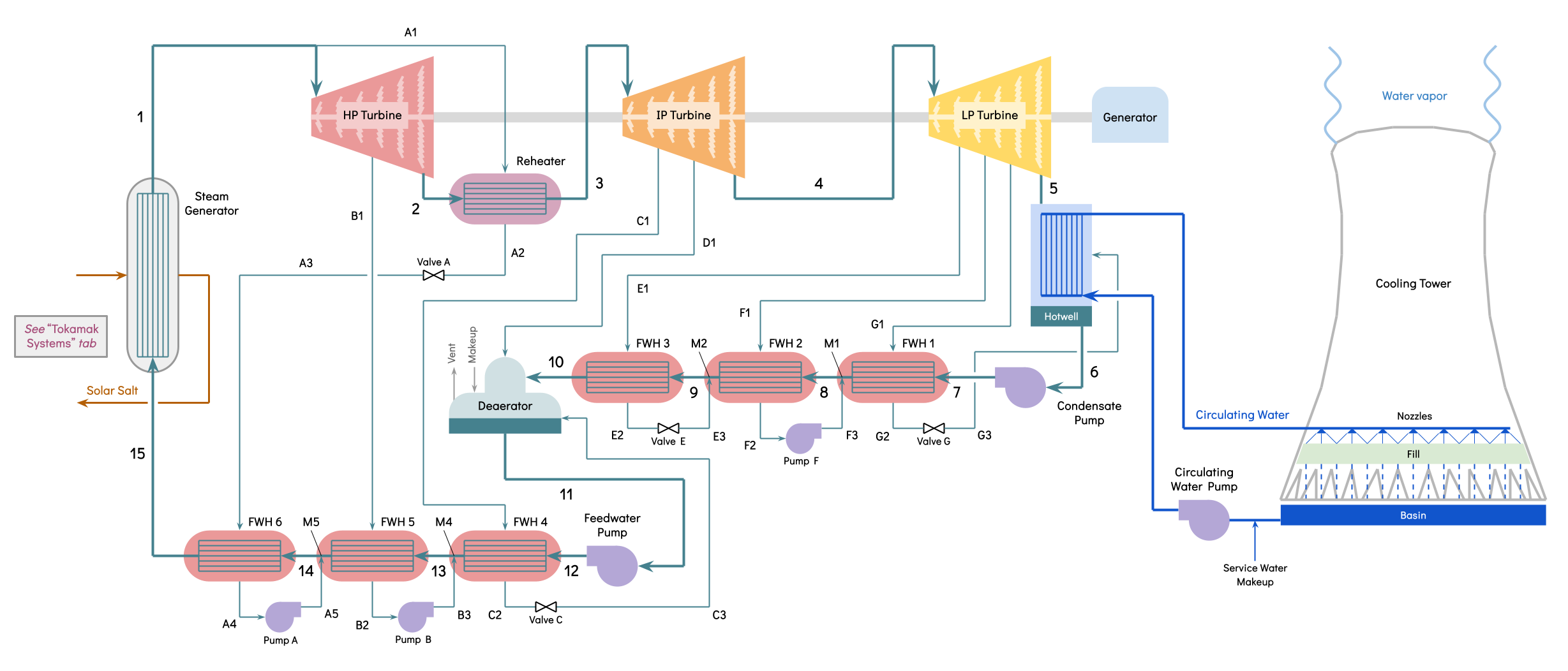
Cycle layout adapted from Colliva, F.; Ciurluini, C.; Iaboni, A.; Centomani, G.V.; Trotta, A.; Giannetti, F. "Analysis of Power Conversion System Options for ARC-like Tokamak Fusion Reactor Balance of Plant." Sustainability 2024, 16, 7480. doi.org/10.3390/su16177480
Modeling Details
Many of the equations used to simulate the Rankine cycle above will look familiar because many are the same equations taught and used analytically in undergraduate thermodynamics courses, derived from the First Law and Second Law. Of course, the complexity of the cycle itself is far higher than any Rankine cycle you would analyze by hand in class. Solving this cycle by hand would be diabolical. Beyond that, I did take some liberties to add some new quirks to make the simulation more realistic, like terminal temperature difference (TTD) for feedwater heaters, dependent condenser pressure, and an empirically-based cooling tower model. All is explained below.
CoolProp calculates properties using mathematical formulas known as equations of state rather than interpolating steam tables. However, the concept that you can determine the rest of the properties of a fluid from two known properties remains the same.
Here are some notation norms used in the sections below: In a general form, a(b, c) is the property "a" when the properies "b" and "c" are known. For example, h(P, T) is enthalpy at a given pressure and temperature. Tsat(P) is the saturation temperature at a given pressure, and hf(P) is the enthalpy of a saturated liquid at that pressure.
Turbines
The turbines are modeled using isentropic efficiency. An ideal turbine expands steam to the exit pressure along a path of constant entropy. A real turbine can be modeled with an isentropic efficiency to account for inevitable losses. You probably already know this:
η = actual work / isentropic work = (hin − hout) / (hin − h2s)
Solving for the actual exit state once the inlet state, exit pressure, and efficiency are known:
h2s = h(Pout, sin)
hout = hin − η·(hin − h2s)
Two different laws are at play here. The actual-work line, hout = hin − η·(hin − h2s), is the First Law steady-flow energy balance for an adiabatic device with negligible KE/PE change, so work out equals the enthalpy drop. The ideal reference state h2s comes from the Second Law. An isentropic (constant-entropy) path is the reversible limit for any adiabatic process, since the real path always generates some entropy (Moran et al., Ch. 6).
Turbine and extraction taps in this cycle:
- HP turbine, state 1 to state 2: h2s = h(P2, s1); h2 = h1 − ηHP·(h1 − h2s)
- HP turbine, extraction B1, state 1 to FWH5: hB1,s = h(PB, s1); hB1 = h1 − ηHP·(h1 − hB1,s)
- IP turbine, state 3 to state 4: h4s = h(P4, s3); h4 = h3 − ηIP·(h3 − h4s)
- IP turbine, extraction C1, state 3 to FWH4: hC1,s = h(PC, s3); hC1 = h3 − ηIP·(h3 − hC1,s)
- IP turbine, extraction D1, state 3 to the deaerator: hD1,s = h(PD, s3); hD1 = h3 − ηIP·(h3 − hD1,s)
- LP turbine, state 4 to state 5: h5s = h(P5, s4); h5 = h4 − ηLP·(h4 − h5s), where P5 = P6, the condenser pressure solved for below
- LP turbine, extraction E1, state 4 to FWH3: hE1,s = h(PE, s4); hE1 = h4 − ηLP·(h4 − hE1,s)
- LP turbine, extraction F1, state 4 to FWH2: hF1,s = h(PF, s4); hF1 = h4 − ηLP·(h4 − hF1,s)
- LP turbine, extraction G1, state 4 to FWH1: hG1,s = h(PG, s4); hG1 = h4 − ηLP·(h4 − hG1,s)
Pumps
Pumps use the mirror image of the turbine equation, using isentropic efficiency. An ideal pump would need less work than a real pump to reach the same exit pressure:
η = isentropic work / actual work = (h2s − hin) / (hout − hin)
h2s = h(Pout, sin)
hout = hin + (h2s − hin) / η
As with the turbines, the actual-work line comes from the First Law energy balance. The ideal reference state h2s is still the Second Law's constant-entropy reversible limit, now for a work-consuming device instead of a work-producing one.
A real plant may use small booster pumps to push a heater's own drain forward into the feedwater line. The governing equation is identical either way.
Pumps in this cycle:
- Condensate pump, state 6 to state 7: h7s = h(Pcondpump, s6); h7 = h6 + (h7s − h6)/ηpump
- Feedwater pump, state 11 to state 12: h12s = h(Pfw, s11); h12 = h11 + (h12s − h11)/ηpump
- Pump A, FWH6 drain A4 to A5: hA5,s = h(Pfw, sA4); hA5 = hA4 + (hA5,s − hA4)/ηpump
- Pump B, FWH5 drain B2 to B3: hB3,s = h(Pfw, sB2); hB3 = hB2 + (hB3,s − hB2)/ηpump
- Pump E, FWH3 drain E2 to E3: hE3,s = h(Pcondpump, sE2); hE3 = hE2 + (hE3,s − hE2)/ηpump
- Pump F, FWH2 drain F2 to F3: hF3,s = h(Pcondpump, sF2); hF3 = hF2 + (hF3,s − hF2)/ηpump
- Circulating water pump, cooling tower basin to condenser inlet and back up to the tower's fill/distribution deck. This cycle uses a natural-draft hyperbolic tower (buoyancy-driven, no fan) rather than a mechanical-draft one - the pump only has to reach the fill deck, not the top of the tower's much taller empty chimney shell above it. There is technically no piping/tower layout modeled, so the head is two generic terms: ΔPcw = ρcw·g·hlift + ΔPref·(ṁcw/ṁref)², a fixed lift (15 m, a typical fill-deck height for a large natural-draft tower) plus a friction term that scales with the square of the actual circulating water flow off a reference point. It responds to the rcw slider and the solved cycle. Then hcw,out,s = h(Pcw,lo+ΔPcw, scw,in); hcw,out = hcw,in + (hcw,out,s − hcw,in)/ηpump. Both anchor figures are generic plant-scale ballparks.
Steam generator (boiler)
A boiler is constant-pressure heat addition with no work done, so the steady-flow energy balance (derived from the First Law, Moran et al., Ch. 4) reduces to heat in per unit mass equals the enthalpy rise:
qin = hout − hin
This simulator sets the boiler's outlet temperature directly instead of solving for it, so the same energy balance is run in reverse. Given the boiler's total thermal duty, the mass flow rate of steam it can support is
ṁ = Q̇ / (h1 − h15), where Q̇ is the duty slider (MW) converted to watts
In this model, the duty arrives from the plant's intermediate loop, which is the solar-salt stream shown in the diagram above. I assume the solar salt enters at 565 °C and leaves at 505 °C (Colliva et al. 2024, Table 1). Note that the Colliva study assumes this fluid is FliBe, however I made a different assumption based on my research. See the "Tokamak Systems" tab for more details. The First Law balance above only cares about the duty and the steam's own states, not that supply temperature, but the Second Law does. See "Cycle performance" below to learn how the intermediate loop sets the exergy limit on what the steam generator can actually deliver. This goes into the Second Law Efficiency calculation.
Condenser
A textbook condenser rejects heat at a constant pressure to a sink at some assumed fixed temperature, with the exit leaving as saturated liquid. The condenser pressure is usually handed to you as a known input. But in the real world, condenser pressure is very much determined by outside factors, so I added some complexity to the modeling of this component. Brace yourself.
This model treats the condenser pressure as a parameter to solve for. So, we employ heat exchanger effectiveness analysis. The solver uses the ε-NTU method, which is a First Law energy balance on both streams combined with a heat transfer rate equation (see Incropera et al., Ch. 11). The two streams are, of course, the condensing steam and the circulating-water loop.
NTU (number of transfer units) is a dimensionless measure of how large the exchanger is relative to the fluid flowing through it. Greater heat transfer area or a smaller flow rate both increase NTU. Effectiveness ε is the fraction of the maximum possible heat transfer the exchanger actually achieves, capped at 1 as NTU increases. In general, ε depends on NTU and the ratio of the two streams' heat capacity rates, Cr. But, because the steam is condensing, it stays at a single temperature across the whole exchanger. This is a special case where one side's heat capacity rate is effectively infinite (Cr approaches 0) which collapses the usual ε-NTU relation to a single exponential (yay):
NTU = UA / (ṁcw·cpcw)
ε = 1 − e−NTU
The heat the condenser must reject and the circulating-water inlet temperature (set by the cooling tower), determine the steam-side saturation temperature. The exit still leaves as saturated liquid because I set it that way, matching the textbook idealization. Since the condenser duty itself depends on the exhaust steam's own state, which depends on the condenser pressure being solved for, this is solved with a trial loop instead of a single formula. The loop re-guesses the condenser temperature T6 each pass until it converges (usually within two or three passes, light work). Every line in the loop below is still just the First Law energy balance on the steam side:
P6 = Psat(T6)
h6 = hf(P6)
h5 = h4 − ηLP·[h4 − h(P6, s4)]
h7 = h6 + [h(Pcondpump, s6) − h6]/ηpump
g = flowFWH1·(h7' − h7) / (hG1 − hG2) (FWH1's extraction fraction, solved here since it needs h7)
flowcond = flowFWH1 − g
Qcond = flowcond·h5 + g·hG2 − flowFWH1·h6
T6,next = Tcw,in + Qcond / (ε·ṁcw·cpcw)
Once converged, the LP exhaust quality is read directly at the exhaust state. If the exhaust steam happens to be superheated instead of wet (possible at a low LP turbine efficiency), its temperature needs its own lookup instead of just reading the saturation temperature:
x5 = quality(P5, h5)
T5 = T6 if x5 ≥ 0 (wet), else T(P5, h5) (superheated)
Cooling tower and circulating water loop
The condenser's cold-side fluid is cooled by an evaporative cooling tower, which relies on mass transfer (water evaporating into air) as much as heat transfer. This means I had to up the complexity of this simulation as well.
Physically, the coldest a cooling tower could ever get the circulating water is the surrounding air's wet-bulb temperature. Real towers can't quite reach that limit, so they're rated by how many degrees above the wet-bulb temperature the cooled water actually leaves at.
Tcw,in = Twb + approach
The wet-bulb temperature itself is found from the ambient dry-bulb temperature T0 and relative humidity RH using an empirical curve fit to measured psychrometric data (Stull, 2011, see Sources), rather than solving the adiabatic-saturation energy balance or reading a psychrometric chart by hand, hence the disgusting formula that follows:
Twb = T0·atan[0.151977·(RH + 8.313659)0.5] + atan(T0 + RH) − atan(RH − 1.676331) + 0.00391838·RH1.5·atan(0.023101·RH) − 4.686035
Specific heat varies slightly with temperature, but the condenser calculation treats it as one constant value throughout rather than tracking it as the circulating water warms up. The constant is evaluated 8°C above the basin temperature, a stand-in for roughly the midpoint of the water's actual rise across the condenser, rather than its coldest point at the inlet:
cpcw = cp(1.5 bar, Tcw,in + 8°C)
Closed feedwater heaters
A textbook closed feedwater heater is a shell-and-tube heat exchanger. Extraction steam condenses on the shell side, giving up its latent heat, while feedwater flows through the tubes.
Feedwater can approach the shell-side saturation temperature but never reach or cross it. A real heat exchanger would need infinite surface area for the feedwater outlet temperature to equal the shell-side saturation temperatue. Terminal temperature difference (TTD) is the practical stand-in for this limit. TTD is the minimum temperature gap a design leaves between the feedwater's outlet temperature and the shell-side saturation temperature.
Ttube,out = Tsat(Pshell) − TTD
htube,out = h(Pfeedwater, Ttube,out)
This part matches the textbook model exactly. Two things are simplified relative to a fully detailed heater:
First, textbook problems often assume the shell-side drain leaves as saturated liquid. This model instead subcools it a fixed amount below saturation, a drain-cooling allowance closer to how a real feedwater heater with an integral drain-cooling zone behaves:
hdrain = hf(Pshell) − ΔTsub·cpf(Pshell), ΔTsub = 2.8°C fixed
Second, rather than modeling desuperheating, condensing, and subcooling as three separate exchanger zones the way a detailed heater design would, each heater here is solved as one lumped energy balance: heat given up by the condensing extraction steam equals the heat picked up by the feedwater, a direct First Law statement (no work, no heat lost to the surroundings) and the same balance behind the standard "extraction fraction" example problem in a thermo course (Moran et al., Ch. 8).
x·(hsteam,in − hdrain,out) = ṁtube·(htube,out − htube,in)
Every closed feedwater heater in this plant, coldest to hottest:
- FWH1, shell pressure PG, heats state 7 (condensate pump outlet) to h7'.
h7' = h(Pcondpump, Tsat(PG) − TTD)
hG2 = hf(PG) − ΔTsub·cpf(PG)
Its drain doesn't get pumped forward: it flashes through Valve G straight into the condenser (see Valves, below). Its extraction fraction g is solved together with the condenser, since it depends on h7, which depends on the converged condenser pressure. - FWH2, shell pressure PF, heats state 8 to h8'.
h8' = h(Pcondpump, Tsat(PF) − TTD)
hF2 = hf(PF) − ΔTsub·cpf(PF)
flowFWH2 = ṁ − a − b − c − d − e
f·(hF1 − hF2 + hF3 − h7') = flowFWH2·(h8' − h7')
Its drain is boosted by Pump F and rejoins at mixer M1, just ahead of its own tube inlet (see Mixing junctions). - FWH3, shell pressure PE, heats state 9 to state 10.
h10 = h(Pcondpump, Tsat(PE) − TTD)
hE2 = hf(PE) − ΔTsub·cpf(PE)
flowFWH3 = ṁ − a − b − c − d
e = flowFWH3·(h10 − h8') / (hE1 − h8')
Its drain is boosted by Pump E and rejoins at mixer M2, ahead of its own tube inlet. - FWH4, shell pressure PC, heats state 12 (feedwater pump outlet).
h12' = h(Pfw, Tsat(PC) − TTD)
hC2 = hf(PC) − ΔTsub·cpf(PC)
c = (ṁ − a − b)·(h12' − h12) / (hC1 − hC2)
Its drain isn't pumped: it's throttled through Valve C straight into the deaerator (see Valves). - FWH5, shell pressure PB, heats state 13 to h13'.
h13' = h(Pfw, Tsat(PB) − TTD)
hB2 = hf(PB) − ΔTsub·cpf(PB)
Its drain is boosted by Pump B and rejoins at mixer M4. FWH5 is coupled to FWH6 and the reheater through streams A and B, so its extraction fraction isn't solved alone, see the Reheater section below. - FWH6, shell pressure PVA, heats state 14 to state 15 (boiler inlet), the hottest heater in the train.
h15 = h(Pfw, Tsat(PVA) − TTD)
hA4 = hf(PVA) − ΔTsub·cpf(PVA)
Unlike the other five, FWH6's steam supply (stream A) is tapped before the HP turbine entirely, not bled from a turbine casing, and its drain is boosted by Pump A and rejoins at mixer M5. See the Reheater section below.
Reheater
Unlike the boiler, the reheater doesn't add heat from an outside source. Its heat comes from stream A: steam tapped off before the HP turbine entirely, never expanded, routed through the reheater's hot side, where it cools while the main HP-exhaust flow on the cold side heats up from state 2 to state 3. Both streams are internal to the cycle, so this is a working-fluid-to-working-fluid heat exchanger, the same kind of energy balance as a closed feedwater heater, not an external heat-addition device like the boiler.
An idealized cycle diagram usually draws every heat exchanger as a constant-pressure process, no friction, no losses. Real tube bundles, headers, and connecting pipe all resist flow, so pressure drops a little every time steam passes through one, the reheater included. That loss doesn't come from either law either, it's a fluid-mechanics effect (friction and minor losses along the flow path), so it's applied here as a simple fixed percentage rather than solved from first principles. The outlet temperature is set directly by the T3 slider:
P3 = P2·(1 − ΔPreheat%)
h3 = h(P3, T3); s3 = s(P3, T3)
Solving streams A and B (FWH5, FWH6, and the reheater together):
Stream A is tapped off before the HP turbine (a1 is exactly state 1, not an expanded bleed), then routed through the reheater's hot side, so it picks up the reheater's duty before reaching FWH6. Stream B is a normal HP turbine bleed feeding FWH5. Because A's flow depends on the reheater's duty, which depends on how much flow is left in the main steam path, which depends on A and B both, these three components are solved together in closed form rather than one at a time:
β = (h13' − h12') / (hB1 − hB2 + hB3 − h12')
R = h3 − h2 (the reheater's enthalpy rise)
a = ṁ·(R + h15 − h13' − β·R) / (h1 + R − h13' − hA4 + hA5 − β·R)
b = (ṁ − a)·β
hA2 = h1 − (ṁ−a−b)·R / a (reheater hot-side outlet, ~P1)
All five of those equations are still just First Law energy balances, three coupled together (reheater, FWH5, FWH6) instead of solved one at a time; nothing here calls on the Second Law directly.
Open feedwater heater (deaerator)
A textbook open (direct-contact) feedwater heater lets the extraction steam and the returning feedwater mix directly, with no tube wall separating them. Because everything mixes together, the outlet always leaves as saturated liquid at the heater's own pressure, no terminal temperature difference needed:
h11 = hf(PD); s11 = sf(PD)
This is exactly the textbook open-feedwater-heater model, unmodified. The plant's one deaerator has three streams mixing into it: the flow arriving from FWH3 (state 10), extraction steam D1 bled directly off the IP turbine, and FWH4's drain after Valve C (C3). Its extraction fraction comes from the same direct-mixing energy balance used in the standard open-feedwater-heater example problem:
flowabc = ṁ − a − b − c
d = [(ṁ−a−b)·h11 − flowabc·h10 − c·hC3] / (hD1 − h10)
Like every mixing calculation on this page, this is conservation of mass paired with the First Law: total mass in equals mass out, and total energy in equals energy out, with no work or heat crossing the boundary.
Throttling valves
A textbook throttle valve is adiabatic, does no work, and has negligible change in kinetic or potential energy, so the First Law leaves enthalpy unchanged across it, one of the cleanest applications of the steady-flow energy balance in the whole cycle (Moran et al., Ch. 4):
hout = hin
Every valve in this plant:
- Valve A, A2 to A3: hA3 = hA2. Drops the reheater hot-side outlet down to FWH6's shell pressure. FWH6's extraction steam is already two-phase by the time it enters the shell, so there's no desuperheating zone.
- Valve C, C2 to C3: hC3 = hC2. Drops FWH4's drain down to the deaerator's pressure, feeding it in directly rather than pumping it forward.
- Valve G, G2 to G3: hG3 = hG2. Drops FWH1's drain down to condenser pressure, flashing part of it to vapor as it enters.
Mixing junctions
Whenever two feedwater streams rejoin, such as a heater's returning drain mixing back into the main feedwater line, the junction is a simple adiabatic control volume with no work: conservation of mass, plus the First Law's conservation of energy, applied at a point, the same mixing-chamber analysis used any time two streams combine in a control-volume problem (Moran et al., Ch. 4).
ṁout·hout = Σ ṁin·hin
Every mixing junction in this plant:
- M1, produces state 8 (FWH2's tube inlet): combines the flow leaving FWH1 (h7', flow flowFWH2 − f) with Pump F's drain (F3, flow f).
h8 = [(flowFWH2 − f)·h7' + f·hF3] / flowFWH2
- M2, produces state 9 (FWH3's tube inlet): combines the flow leaving FWH2 (h8') with Pump E's drain (E3, flow e). Solved together with FWH3's own heating balance:
h9 = h10 − e·(hE1 − hE2) / flowFWH3
- The deaerator itself produces state 11 the same way (it's an open feedwater heater, so mixing is its whole job) - the numbering just skips from M2 to M4 because the deaerator isn't a separate M3 node in the code, it is the mixing point. Described under "Open feedwater heater" above.
- M4, produces state 13 (FWH5's tube inlet): combines the flow leaving FWH4 with Pump B's drain (B3, flow b), flow (ṁ−a) total. Streams A and B are solved together in closed form (see the Reheater section above), so the coded formula is expressed via FWH5's own outlet h13' rather than FWH4's directly, but it's the same mixing point:
h13 = h13' − b·(hB1 − hB2) / (ṁ − a)
- M5, produces state 14 (FWH6's tube inlet): combines the flow leaving FWH5 (h13', flow ṁ−a) with Pump A's drain (A5, flow a).
h14 = [(ṁ − a)·h13' + a·hA5] / ṁ
Generator
Not a thermodynamic control volume at all, and not derived from either law: just a real-world mechanical-to-electrical conversion efficiency that most idealized cycle problems skip entirely, since the shaft work the turbines produce isn't all delivered as electricity.
Wnet = (Wturbines − Wpumps)·ηgenerator
Cycle performance
The first-law (thermal) efficiency is the same Rankine-cycle efficiency definition from any thermodynamics textbook: net work out divided by heat in, straight from conservation of energy (Moran et al., Ch. 8).
η1st law = Wnet / Q̇
The second-law (exergetic) efficiency compares the net work out to the exergy, or maximum possible work, that was actually available to extract. Exergy is the flow-availability function from the second-law chapter of a thermo course, measured relative to a fixed ambient dead state (h0, s0, T0), and it exists as a concept at all because of the Second Law: no real process can convert 100% of a heat input into work, so exergy tracks the upper bound that's actually achievable rather than the full energy content (Moran et al., Ch. 7):
ψ = (h − h0) − T0·(s − s0)
Applied across the boiler, the dead-state terms cancel out of the difference, leaving the exergy the steam itself gains:
Exsteam = ṁ·[(h1 − h15) − T0·(s1 − s15)]
Exsteam only sees the steam's own states, so it has no way to notice how irreversibly that heat was actually delivered - a slider change that forces the boiler to heat much colder feedwater (e.g. bypassing every FWH) can make Wnet / Exsteam look better even though the plant is strictly worse, because cutting the FWHs' own mixing losses can outweigh the (invisible, to Exsteam) extra irreversibility of the wider-ΔT boiler heat exchange.
Plain first-law efficiency never has this loophole - Q̇ is Q̇ no matter how it's delivered - which is why a whole-plant second-law efficiency is conventionally referenced against the exergy of the resource actually supplying the heat, not the exergy of whatever happens to receive it (Moran et al., Ch. 7, draws exactly this distinction between a component's own second-law efficiency and a plant's, which is referenced to its fuel or heat source). Pricing the same heat against the intermediate loop's own temperature glide fixes it here. The exergy a stream gives up delivering heat δQ at its own local temperature T is (1 − T0/T)·δQ, so integrating over the intermediate loop's full cooldown from Tin to Tout gives the total exergy it gives up:
Exsource = ∫ (1 − T0/T)·δQ̇, integrated from Tin to Tout
For a stream of roughly constant cp (a fair assumption for solar salt over a 60 °C span with no phase change), δQ̇ = −ṁcp·dT, and that integral works out in closed form to Q̇·(1 − T0/Tlm), where Tlm is the log-mean (entropic-average, not arithmetic-average) temperature - the same log-mean-temperature-difference logic from a heat-transfer course, applied here to exergy instead of heat rate. This needs only the two supply/return temperatures and the duty, not the stream's mass flow or its actual cp value:
Tlm = (Tin − Tout) / ln(Tin/Tout)
Exsource = Q̇·(1 − T0/Tlm)
Tin and Tout are the intermediate (solar-salt) loop's own supply and return temperatures at the steam generator: 565 °C and 505 °C (Colliva et al. 2024, Table 1 - the source paper's own intermediate fluid is FLiBe rather than solar salt, but its supply/return temperatures are what this plant's secondary heat exchangers are sized to, regardless of which fluid carries them; see the sources list). That puts Tlm at 807.7 K (534.6 °C) and the Carnot factor 1 − T0/Tlm at 0.631 for a 25 °C ambient - the ceiling every cycle's second-law efficiency is measured against below. Exsource doesn't depend on any steam-side slider at all, only on Q̇ and ambient T0, so it can't be gamed by changing how the feedwater arrives. Second-law efficiency is computed against it instead of Exsteam:
η2nd law = Wnet / Exsource
T0 is the ambient temperature (in kelvin). This splits the total exergy destroyed into two pieces: how much was lost transferring heat from the primary loop into the steam itself (a real irreversibility this model didn't track at all before), and how much was lost downstream of that, in the turbines, condenser, pumps, and FWH mixing:
Irrsteam generator = Exsource − Exsteam
Irrcycle = Exsteam − Wnet
Both are pure Second Law quantities, each proportional to the entropy generated in its own piece of the plant (the Gouy-Stodola theorem, Irr = T0·Sgen), and the Second Law guarantees neither can come out negative, no matter how the sliders are set. Total exergy destroyed, consistent with η2nd law, is just their sum:
Irr = Exsource − Wnet = Irrsteam generator + Irrcycle
Every monitoring value on the dashboard
The gauges, readout cards, and the condenser helper line above are all built from the component equations already given. This lists each displayed value by its exact label and its formula, so any number on the dashboard can be traced back to how it was found.
Gauges
- 1st law efficiency: η1st law = Wnet / Q̇
- 2nd law efficiency: η2nd law = Wnet / Exsource
- LP exhaust quality: x5, or 1 (full quality) if the exhaust came out superheated instead of wet
- Pump power fraction: Wpumps / Wturbines
Readout cards
- Net electrical output: Wnet = (Wturbines − Wpumps)·ηgenerator
- Turbine work: Wturbines = WHP + WIP + WLP, the sum of each turbine section's own work
WHP = (ṁ−a)·h1 − (ṁ−a−b)·h2 − b·hB1
WIP = (ṁ−a−b)·h3 − (ṁ−a−b−c−d)·h4 − c·hC1 − d·hD1
WLP = (ṁ−a−b−c−d)·h4 − flowcond·h5 − e·hE1 − f·hF1 − g·hG1
- Feedwater pump power: Wfwp = (ṁ−a−b)·(h12 − h11)
- Condensate pump power: Wcondpump = flowFWH1·(h7 − h6)
- Circulating pump power: Wcwpump = ṁcw·(hcw,out − hcw,in)
- Exergy to working fluid: Exsteam = ṁ·[(h1 − h15) − T0·(s1 − s15)]
- Total steam flow: ṁ = Q̇ / (h1 − h15)
- Circulating water flow: ṁcw = rcw·ṁ, where rcw is the circulating-water-to-steam mass ratio slider
- Condenser pressure: P6 = Psat(T6), the converged condenser saturation pressure from the trial loop above
- Condenser TTD: TTDcond,eff = T6 − Tcw,out, where Tcw,out = Tcw,in + Qcond/(ṁcw·cpcw)
- Hotwell temperature: T6, the converged condenser saturation temperature
- Cooling tower basin temp: Tcw,in = Twb + approach
Condenser helper line (shown under the Cooling / Environment sliders)
- NTU: NTU = UA / (ṁcw·cpcw)
- ε: ε = 1 − e−NTU
- Range: ΔTcw = Qcond / (ṁcw·cpcw), the circulating-water temperature rise across the condenser
- TTD: same as the condenser TTD readout card above
Sources
The component models above follow standard undergraduate thermodynamics and heat-transfer texts. Steam properties come from the IAPWS-95 formulation, accessed through CoolProp.
- M. J. Moran, H. N. Shapiro, D. D. Boettner, M. B. Bailey, Fundamentals of Engineering Thermodynamics, 8th ed., Wiley. Turbine and pump isentropic efficiency, the Rankine cycle, open and closed feedwater heaters, throttling valves, and mixing chambers (Ch. 4-6, 8); exergy analysis (Ch. 7).
- Y. A. Çengel, M. A. Boles, Thermodynamics: An Engineering Approach. Alternate standard reference for the same topics.
- F. P. Incropera, D. P. DeWitt, T. L. Bergman, A. S. Lavine, Fundamentals of Heat and Mass Transfer. The ε-NTU heat-exchanger effectiveness method used for the condenser.
- R. Stull, "Wet-Bulb Temperature from Relative Humidity and Air Temperature," Journal of Applied Meteorology and Climatology 50, 2267-2269 (2011). The wet-bulb correlation used for the cooling tower.
- W. Wagner, A. Pruß, "The IAPWS Formulation 1995 for the Thermodynamic Properties of Ordinary Water Substance for General and Scientific Use," Journal of Physical and Chemical Reference Data 31, 387-535 (2002). The steam-table property source for every enthalpy, entropy, and temperature lookup in this model.
- I. H. Bell, J. Wronski, S. Quoilin, V. Lemort, "Pure and Pseudo-pure Fluid Thermophysical Property Evaluation and the Open-Source Thermophysical Property Library CoolProp," Industrial & Engineering Chemistry Research 53(6), 2498-2508 (2014). The software library implementing IAPWS-95 that every property lookup in this simulator runs through.
- F. Colliva, C. Ciurluini, A. Iaboni, G. V. Centomani, A. Trotta, F. Giannetti, "Analysis of Power Conversion System Options for ARC-like Tokamak Fusion Reactor Balance of Plant," Sustainability 16, 7480 (2024). This cycle's layout, extraction pressures, and operating conditions; the intermediate loop's 565/505 °C supply/return and 645 MWth duty, shared by all three power conversion cycles on this site. That paper's own intermediate fluid is FLiBe rather than the solar salt used here - the temperatures and duty still apply (see the MANTA reference below), but its stated 1500 kg/s intermediate mass flow is per primary train (there are three) and isn't the figure this site's solar-salt loop would use, since FLiBe and solar salt have different heat capacities.
- MANTA Collaboration, "MANTA: A Negative-Triangularity NASEM-Compliant Fusion Pilot Plant," arXiv:2405.20243 (2024). The choice of 60% NaNO3/40% KNO3 solar salt as the intermediate loop's working fluid, selected so its boiling and recrystallization points bracket both heat exchangers' hot and cold legs.
- F. Colliva et al., "Conceptual design and supporting analysis of a Double Wall Heat Exchanger for an ARC-class fusion reactor Primary Cooling System," Fusion Engineering and Design 201, 114261 (2024). Background on the FLiBe primary loop and blanket-side double-wall heat exchanger, upstream of everything this simulator actually models - it's mentioned above only for context on why the intermediate loop exists as a separate stream.